What is a neural network?

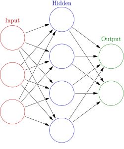
The term Neural Network was coined as far back as 1943 by McCulloch and Pitts. They were inspired by the way the human brain works. Now a days, neural networks come in different shapes and forms. It can either look like this (Feed Forward Fully Connected Network)

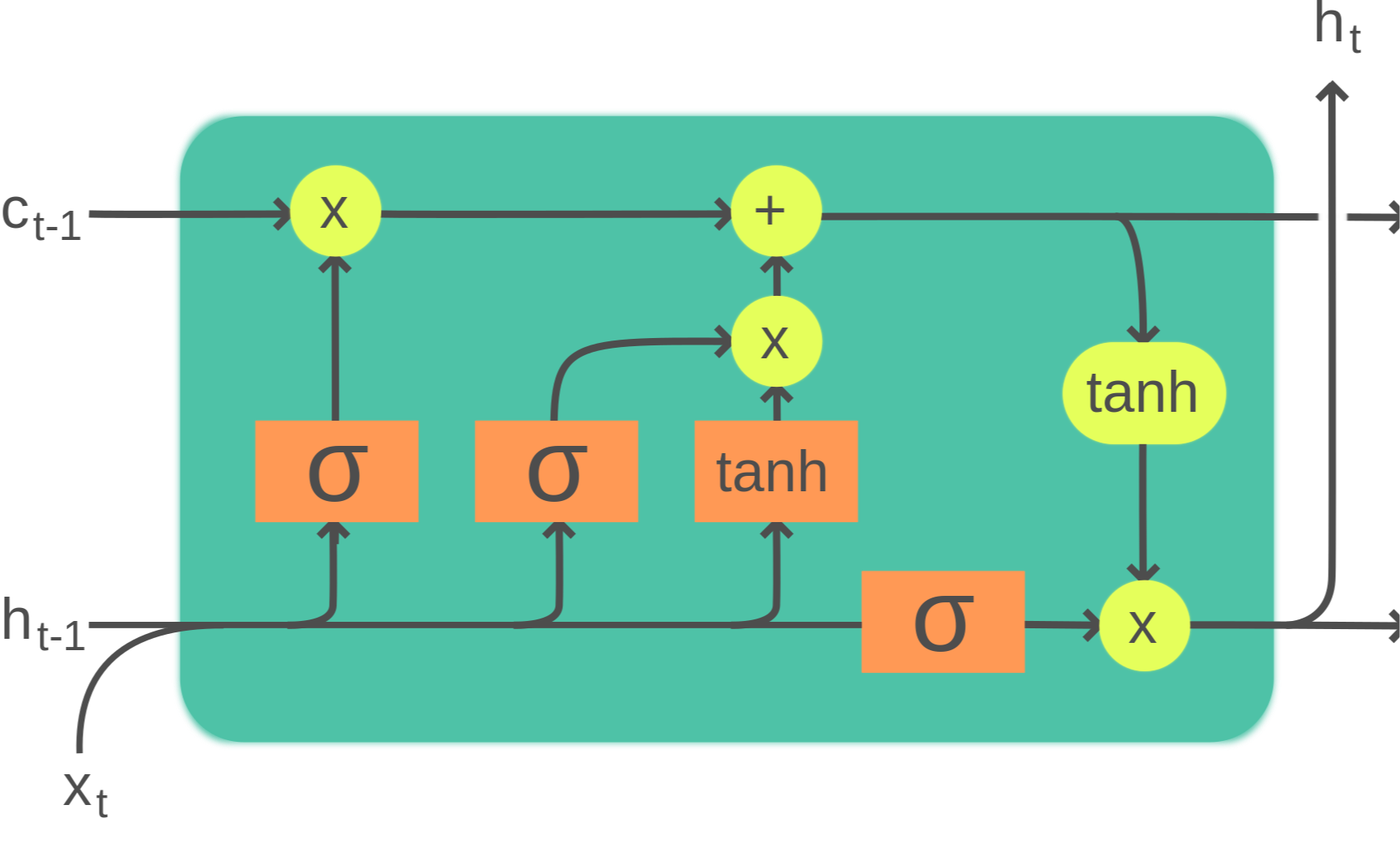
or it can look like this (LSTM Cell of RNN Architecture)

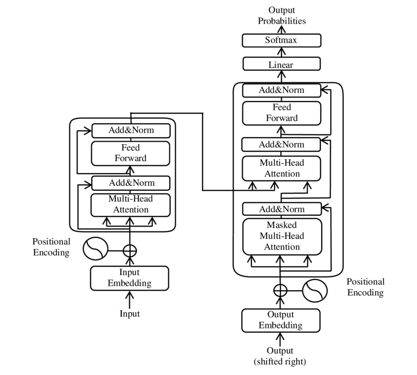
or it can look like this (Transformer Architecture)

One thing that is common between these architectures is that we have some data, and we expect these architectures to learn some patterns in the data. The data can be anything from images, text, audio, video, etc. The patterns can be anything from recognizing a cat in an image, to predicting the next word in a sentence, to generating a new image from a given image, etc. Lets try to understand how these architectures learn. One of the components of learning is to define an objective, or a loss function.

Lets build an intuition of the Loss Function

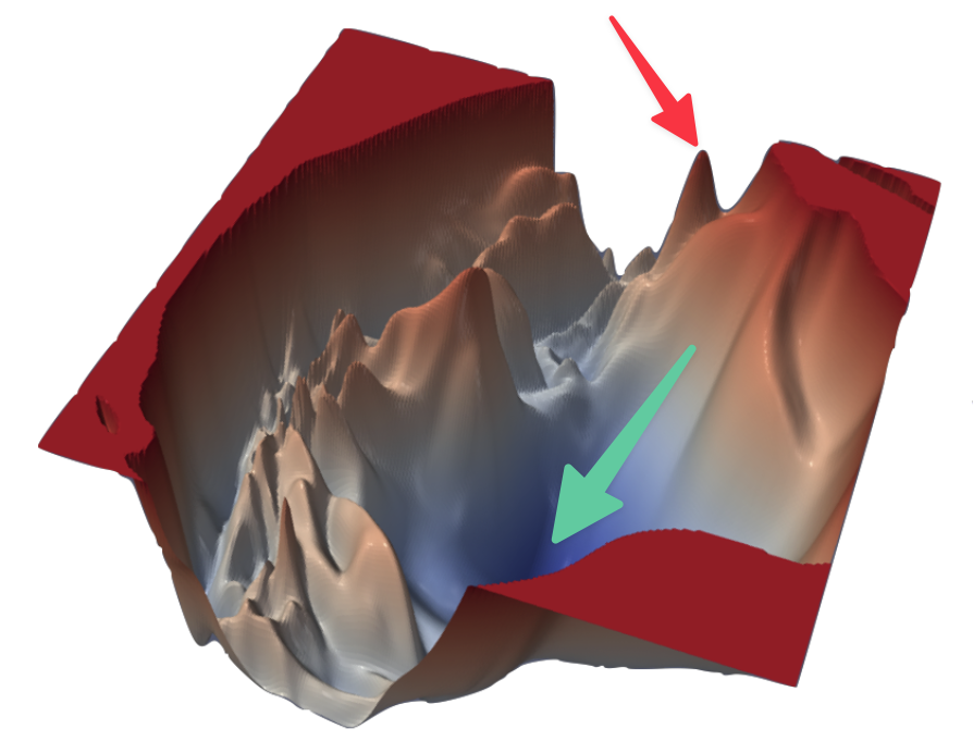
When we humans have a clearly defined goal, and we take actions which take us closer to that goal with every step of the action, we call that effective learning. Neural Networks which are powering today's advancements on Deep Learning and AI learn on a similar principle. We define an objective or a goal which we want the network to get better at. Lets try to build a visual intuition into how does that objective looks like.

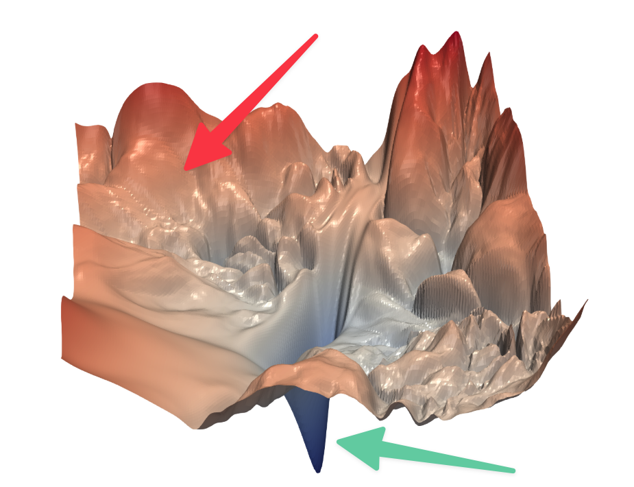
Visualizing the Loss Landscape of Neural Nets - Li et. al., 2017

Imagine yourself standing on a ragged terrain pictured above. Imagine yourself somewhere near where the red arrow is pointing and you want to reach someplace where the green arrow is pointing. You are also blindfolded and there is no way for you to know which direction to move. The only thing you can do is to take an action. Every time you take that action, a mysterious power comes and moves you slightly in the correct direction towards the green arrow. This is essentially the mechanism of neural network training.

The mysterious power that I mentioned above is called "Back Propagation". Backprop essentially helps the network state (the coordinates where you were standing on the terrain can be called a state) move slightly to a state which helps it get better at the task. So, to summarise, every neural network learning involves an objective or a loss function. Lets take a simple example and see how it works.

Consider an objective, where you wish to train a network to regenerate an image of a cat, i.e the network should look at an image of a cat, and output an image with same features. How would you know quantitatively whether the network succeded in its objective or not? A simple way can be to take pixel wise squared distance of both the images and try to minimise it. Mathematically, we can say that

$$\mathcal{L}(x_i, y_i; \theta) = \sum_{p=1}^P (x_i^{(p)} - y_i^{(p)})^2$$

This is just a fancy way to formulate that we want to make the regenerated image as close to the original image as possible. $x_i^{(p)}$ means pixel $p$ of image $i$. Lets stare at this equation for a bit. What does it have to do with learning and training. We can think of this like a dart game. You get better point if you hit the target near the Bull's Eye. This mathematical formulation of the equation is some sort of number which depicts how good is the network at any given point of time in its learning journey. I hope it is well received till this point, that in order for the network to get better, we need to bring the value of the equation down. How to do this? The answer is the work horse of every AI practitioner, Gradient Descent.

Lets look at the image given below. At every step, the slope or gradient points upwards, and we take a small step opposite to the slope. Effectively this brings us to a state in the curve, which has minimum value.

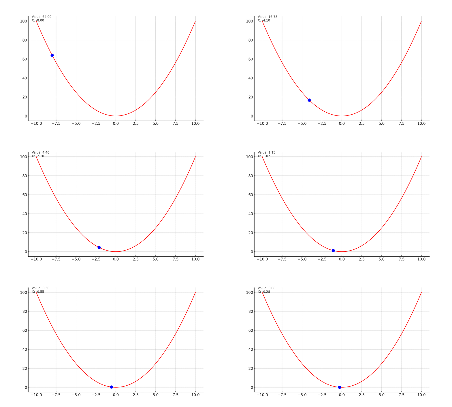
Mathematically, we are updating the state of the network with every time stap. $$\theta_t = \theta_{t-1} - \alpha * \nabla_{\theta} \mathcal{L}(x_i, y_i; \theta)$$

Now that we have an basic intuition of what a loss function is, lets go to the next step.

How to choose the objective?

This is sort of where science meets art. Why did we choose sum of squared distance as our objective and not sum of absolute distance. In other words, why did we not consider

$$\mathcal{L}(x_i, y_i; \theta) = \sum_{p=1}^P ||x_i^{(p)} - y_i^{(p)}||$$

Take current state of the art LLMs for instance. BERT learns by predicting masked tokens and next sentence of text input. Example: consider two sentences - "artificial intelligence in its broadest sense is intelligence exhibited by machines" and "it is a field of research in computer science". We would give the sentence to BERT model "artificial [MASK] in its [MASK] sense is intelligence [MASK] by machines" and if the output is "intelligence", "broadest" and "exhibited", we say that the loss is close to 0, or the Neural Network did well. If it is also able to predict that next sentence has a good probability of occuring as a next sentence, it did well. While GPT uses the next word prediction. We will feed in "artificial intelligence in its broadest sense is" as input, and we should have "intelligence" as the ouput for us to say that the network did well. Both of these LLMs are able to learn about our world with very different objectives. This is not very different to how we would try to achieve certain goals in real life, like some companies may focus on their Marketing Campaigns to increase sales for their business while some companies may double down on their Product Innovation. You can find descent arguments for both of these approaches.

What are the problems that we can formulate with the help of such mathematical objectives?

I like to think it as below. Consider a function $y = \mathcal{D}(x)$. You have inputs $x$ and you have outputs $y$. But you have no idea on how $\mathcal{D}$ looks like. Let's take a well known problem of Sentiment Classification. Given an input statement $x_1$, "I loved the movie", the function $\mathcal{D}$ should output 1 (positive sentiment) and an input statement $x_2$, "What a waste of time", the function $\mathcal{D}$ should output 0 (negative sentiment). The problem is pretty easy to describe, but we have no idea how to formulate the function or write logic for it. Lets throw in some neural network. We don't need to bother about $\mathcal{D}$ now. We just need to define an objective. Take below formulation for example

$$\mathcal{L}(x_i, y_i; \theta) = - y_i\log{(\mathcal{D}(x_i; \theta))} - (1 - y_i)\log{(1 - \mathcal{D}(x_i; \theta))}$$

Think about what happens when the model outputs the correct answer, i.e when true label is 1 and model outputs 1 or when true label is 0 and model outputs 0. [ Hint: $\log(1) = 0$]. So, we can see that we have very smartly formulated an objective and need not worry at all about the function that we had to learn. We can learn any $\mathcal{D}$ as long as we have enough compute and data and have come up with a clever way to formulate an objective.

Hope this helped you gain some intuition into how we design and train the neural network architectures. If you have some followup posts I should write or have some comments, please feel free to comment below.

References

1. If you wish to know about Back Propagation in more depth, checkout CS231 Notes and Andrej's blog
2. LSTM Cell Image and Transformer image taken from Wikipedia